Decision Trees
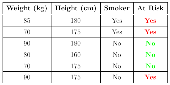
Decision trees are simple, versatile learning algorithms that form the base of several more sophisticated algorithms such as random forests and gradient boosted models. Decision trees work by partitioning the feature space through one or more decision splits. For example, consider the following simple (and entirely fictional) dataset indicating if someone is at risk of heart disease or not along with their height, weight and whether or not they are a smoker.
Based on this we could construct a decision tree which will correctly classify all the instances in this dataset as ‘at risk’ or ‘not at risk’ of heart disease:
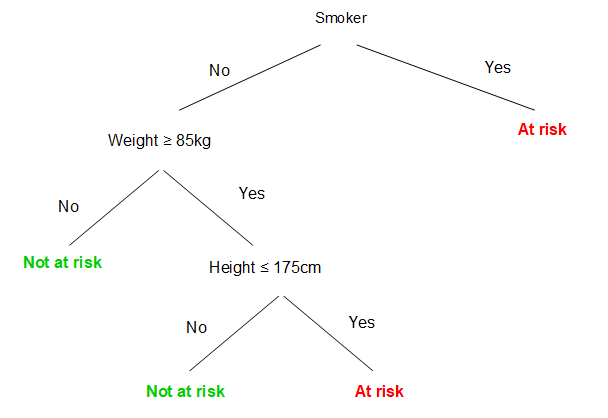
The root node is the top node containing all of the data before it has been split. Each subsequent node that partitions the data is known as a decision node (sometimes also referred to as a split node, alternate node or just node). The final nodes that have no additional nodes coming off them are the leaf nodes.
After constructing the tree using our training data, we could then use it make predictions on new data simply by navigating from the top of the tree downwards until we reach a leaf node.
Training a Decision Tree
There are many algorithms available for training a decision tree (sometimes referred to as growing the tree). Here we will focus on the commonly used CART (Classification And Regression Tree) algorithm, which performs a series of binary splits on the data until some stopping criteria is reached.
Splitting criteria
Each step of the tree-growing process must select a test condition to divide the data into smaller subsets. In other words, the algorithm needs to decide on the best ‘question’ to ask at each split point. To select the optimal condition the algorithm needs an objective measure for evaluating the goodness of a split. The choice of measure differs depending on whether the objective is classification or regression.
In a classification tree, the goal is to separate the classes. A good split, therefore, is one that divides the classes into more ‘pure’ subsets. CART trees use the gini impurity as a measure of the impurity of a set:
\[Gini \space impurity = 1 - \sum_{k=1}^{n}p_{k}^2\]where \(p\) is the ratio of instances belonging to class \(k\) in the node, and n is the number of classes. This is a measure of how often a randomly chosen element from a set would be incorrectly labelled if it was randomly labelled according to the distribution of labels in the subset.
To make this clearer, let’s take an example from the fictional heart disease dataset presented earlier. The dataset contains two classes: ‘at risk’ and ‘not at risk’, which we will refer to as positive and negative instances respectively. The initial, untouched dataset has an even number of positive and negative instances. Therefore, if we were to select an instance at random the probability of getting a positive instance would be 0.5, and the probability of getting a negative instance would also be 0.5. The gini impurity would therefore be: \(1 - (0.5^2 + 0.5^2) = 0.5\).
After splitting the data into sets of smokers and non smokers, the gini impurity of the ‘smoker’ node would be \(1 - (1^2 + 0^2) = 0\), while the gini impurity of the ‘non smoker’ node would be \(1 - (\frac{1}{3}^2 + \frac{1}{4}^2) = \frac{3}{8} =0.375\).
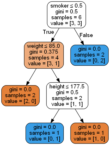 Visualisation of the entire tree fit using the scikit-learn library
CART is a greedy algorithm, it tries all choices of feature and feature value contained in the dataset and chooses the one that minimises the gini impurity. Note that the algorithm is only computing the optimum split at that node; finding the global optimum for a tree is computationally infeasible.
In a regression tree, the algorithm works in much the same way, except that instead of trying to split the training set to best minimize the impurity, it now tries to split the training set to best minimize the mean-squared-error. The decision node aims to split the data in order to minimize the sum of the differences between each sample in the node and the mean value of samples in the node. So, for a split resulting in two nodes \(n_1\) and \(n_2\) containing a combined total of \(m\) training instances:
\[J(n_1, n_2) = \frac{m_{1}}{m}\sum_{i\in n_1}(y^{(i)} - \overline{y}_{n_1})^2 + \frac{m_{2}}{m}\sum_{i\in n_2}(y^{(i)} - \overline{y}_{n_2})^2\]Early stopping Criteria
A decision tree can be grown until it perfectly fits the entire data set. However, in reality, this is usually not desirable as it will result in an overfitted tree which doesn’t generalise well to new data. To prevent this, criterion can be specified to stop the algorithm early. For example the tree growing process could stop when:
- The tree reaches a specified maximum depth.
- The impurity (or mean-squared-error in the regression case) decrease from a split is below a specified threshold.
- The number of training examples in a node drops below a certain threshold.
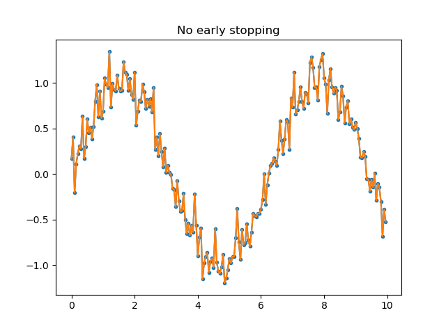
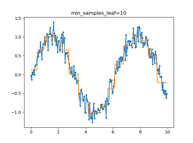
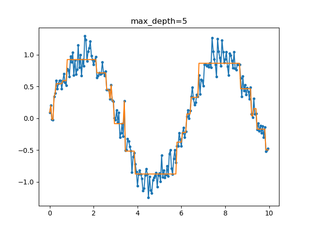
To illustrate how early stopping can prevent overfitting, the following figures show the results of fitting decision trees to a \(sin\) function + random noise. The tree fit without early stopping is clearly overfitting (fitting to the random noise) very badly. Setting limits on the minimum number of samples in a leaf or the maximum tree depth results in a much more reasonable model.
Advantages and Disadvantages of Decision Trees
Decision trees have several advantages:
- The trees are easily visualised and interpreted, it’s easy to see exactly how the algorithm came up with the result for a particular instance (especially true for small trees).
- They can trivially handle both continuous and categorical input data.
- They can be used for both classification and regression tasks.
- They are nonparametric i.e. they do not require any prior assumptions about the distribution of the data.
- They are generally robust to outliers
- They perform implicit feature selection and the presence of redundant features does not adversely affect the performance of the decision tree.
However, they are not without disadvantages:
- Decision trees are extremely susceptible to overfitting, creating over-complex trees that do not generalise the data well. This can be mitigated somewhat by using early stopping criteria.
- They are very sensitive to small variations in the data, making them highly unstable.
- Since all the decisions are made using a single feature, decision trees have orthogonal decision boundaries. This makes them sensitive to training set rotation.