Logistic Regression

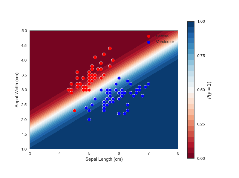
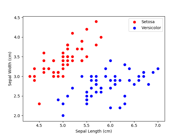
Logistic Regression is linear algorithm for classification tasks. It outputs the probability that an instance belongs to a particular class. If the model outputs a probability greater than 0.5, the model will predict that the instance belongs to that class. In the later sections of this article we will use data from the classic Iris flower data set (https://en.wikipedia.org/wiki/Iris_flower_data_set). Our objective will be to classify if a flower is of the species ‘Setosa’ or ‘Versicolor’ based on the length and width of the sepals.

Like Linear Regression, a Logistic Regression model calculates a weighted sum of input features (plus a bias term):

where \(\theta\) is the vector of coefficients and \(x\) is the vector of input features (independent variables).

However, unlike the linear regression, this weighted sum of input features must be transformed into a probability. Therefore, the output p must be constrained to be between 0 and 1, since a probability cannot be negative or greater than 1. A function that satisfies these conditions is the logistic function (also referred to a the logit):

This is a sigmoid (i.e. S-shaped) function that outputs a number between 0 and 1:

Just as with Linear Regression, we need a quantitative measure of good (or bad) the model is. Again, we need a cost function. The objective is to set the parameters so that the model will estimate high probabilities for positive instances (the instance belongs to a particular class) and low probabilities for negative instances (the instance does not belong to a particular class). We can accomplish this using the following cost function:

To understand why this works as a cost function, consider what happens for positive and negative instances. In the positive case, the function becomes: \(J=-log(p)\)

As \(p\) increases the cost decreases. We want large \(p\) for positive instances. The negative case is of course the reverse:

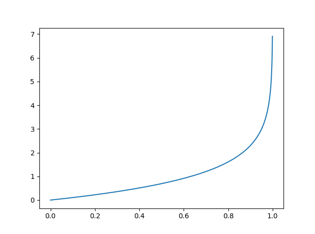As \(p\) increases, the cost increases. We want small \(p\)for negative instances.

This cost function has the advantage that it is convex, so an optimization algorithm such as gradient descent is guaranteed to find the global minimum (given an appropriate learning rate and enough time). So, we can train a logistic regression model using gradient descent. For this, we need to calculate the derivative of the cost function:

Python implementation of Logistic Regression

class LogisticRegression:

    def __init__(self, learning_rate=0.001, epochs=1000):
        self.theta = None
        self.learning_rate = learning_rate
        self.epochs = epochs

    def sigmoid(self, x):
        return 1/(1+np.exp(-x))

    def predict_probability(self, X, theta):
        return self.sigmoid(np.dot(X, theta))


def stochastic_gradient_descent(self, X, y):
    # Add intercept to input data
    intercept = np.ones((X.shape[0], 1))
    X = np.concatenate((intercept, X), axis=1)
    theta = np.zeros(X.shape[1])

    for _ in range(self.epochs):
      # Update theta
      for ix in range(X.shape[0]):
          proba_prediction = self.predict_probability(X[ix], theta)
          gradient = np.dot((proba_prediction - y[ix]), X[ix])
          theta = theta - (gradient * self.learning_rate)

  return theta


def fit(self, X, y):
  self.theta = self.stochastic_gradient_descent(X, y)


def predict_proba(self, X):
  intercept = np.ones((X.shape[0], 1))
  X = np.concatenate((intercept, X), axis=1)

  return np.array([self.predict_probability(self.theta, x) for x in X])


def predict(self, X):
  proba_predictions = self.predict_proba(X)

  return [1 if proba >= 0.5 else 0 for proba in proba_predictions]

We can use now fit a logistic regression model to the Iris data. Visualising the model we can see the decision boundary almost perfectly separates the flower types: