Regularised Regression

Regularised Regression

Regularisation is a technique that constrains a model. For linear models regularization is usually achieved by shrinking the values of the coefficients or setting some coefficient to zero. There are two reasons why this may be advantageous compared to the vanilla least squares approach. Firstly, regularisation can reduce the bias of the model, reducing the risk of overfitting and potentially improving the predictive accuracy of the model. Secondly, regularisation can improve the interpretability of the model by identifying the predictors that are most relevant.

The three main regularisation algorithms for linear models are: Ridge Regression, Lasso Regression and Elastic Net. In each of these algorithms, a regularisation term is added to the cost function that forces the algorithm to keep the weights as small as possible.

Ridge regression penalises large weights by adding the L2 norm to the cost function.

\[J(\theta) = MSE(\theta) + \alpha \frac{1}{2} \sum_{i=1}^{n} \theta_{i}^2\]

Here \(\alpha\) is a regularisation parameter which controls the amount of shrinkage, the larger the value of \(\alpha\) the greater the shrinkage.

Lasso regression also penalises weights but uses the L1 norm:

\[J(\theta) = MSE(\theta) + \alpha \frac{1}{2} \sum_{i=1}^{n} \left|\theta_{i}\right|\]

Note that while the ridge cost function is differentiable everywhere, the lasso cost function is not differentiable at 0. Therefore, gradient descent can not be used to minimize this function. Instead, we can use variations of coordinate descent and utilize notions from subdifferential theory (see later section on deriving the lasso update).

Elastic Net is a compromise between ridge and lasso regression which uses a mix of both the L1 and L2 norm:

\[J(\theta) = MSE(\theta) + \lambda \alpha \frac{1}{2} \sum_{i=1}^{n} \left|\theta_{i}\right| + (1-\lambda)\alpha\sum_{i=1}^{n} \theta_{i}^2\]

Here \(\lambda\) is a mixing parameter which controls the relative importance of the L1 and L2 penalties.

Comparison of Lasso, Ridge and Elastic Net

While both lasso and ridge regularisation provides shrinkage, they behave quite differently in practice.

The coefficients in a ridge model can approach zero but will never be completely removed. Lasso, on the other hand, can produce sparse solutions by shrinking coefficients all the way to zero. For example, the following figures show the coefficient paths for ridge and lasso models on the Boston housing dataset (https://www.kaggle.com/c/boston-housing):

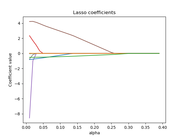
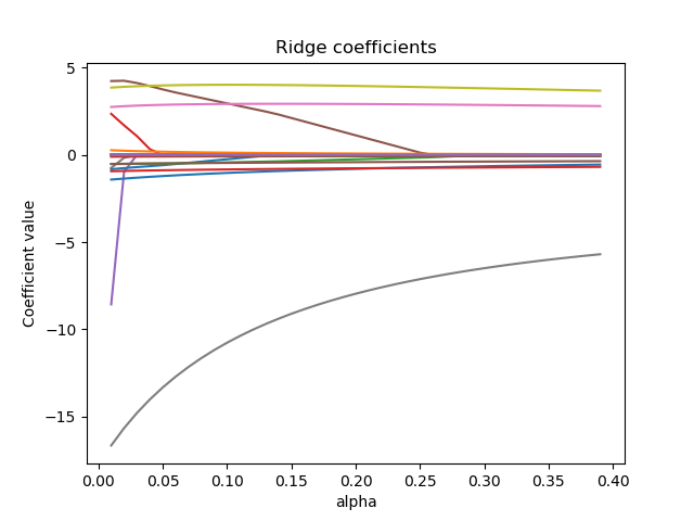
Ridge regression shrinks highly correlated variables together, while lasso tends to pick one and ignore the others. In the extreme case of \(m\) perfectly correlated features, ridge would produce a model with all the coefficients equal to \(1/m\). Lasso, on the other hand, would select one feature at random and drop the rest.

Elastic net offers a useful compromise between the lasso and ridge, since it selects variables like the lasso, and shrinks together the coefficients of correlated predictors like ridge. However, it does have an additional hyperparameter (the mixing parameter between the L1 and L2 penalties) that needs to be tuned.

Deriving the lasso coordinate descent update using Subgradients

Coordinate descent algorithms are iterative methods in which each update step is obtained by fixing most components of the independent variable vector at their current values and then approximately minimising with respect to the remaining variables.

Our aim is to minimize the lasso cost function:

\[J(\theta) = \large\sum_{i=1}^{N}\Bigl(\small\frac{1}{2}(y^{(i)}-\sum_{m=1}^{M}\theta_{m}x_{m}^{(i)})^{2} + \alpha \sum_{m=1}^{M} \left|\theta_{m}\right|\Bigl)\]

To do this, we take the partial with respect to \(\theta_{m}\) with all other weights fixed, then set this to 0. We’ll start with the mean squared error term, then deal with the penalty term.

\[\frac{\partial MSE}{\partial \theta_m} = \large\sum_{i=1}^{N}(\small -x_{m}^{(i)}(y^{(i)}-\sum_{m=1}^{M}\theta_{m}x_{m}^{(i)})\bigl)\]

We can then split out the \(\theta_{m}\) from all other weights in the summation:

\[\begin{aligned} \frac{\partial MSE}{\partial \theta_m} = & \large\sum_{i=1}^{N}(\small - x_{m}^{(i)}y^{(i)} + x_{m}\sum_{k\neq m}^{M}\theta_{k}x_{k}^{(i)} + \theta_{m}x_{m}^{2(i)}\bigl) \\ = & \large\sum_{i=1}^{N}(\small -x_{m}^{(i)}y^{(i)} + x_{m}\sum_{k\neq m}^{M}\theta_{k}x_{k}^{(i)} + \theta_{m}x_{m}^{2(i)}\bigl) \\ = & -\rho_{m} + \theta_{m} z_{m} \end{aligned}\]

We can then move on to the penalty term. At \(\theta_{m}<0\) and \(\theta_{m}>0\) the gradient is clearly \(-\alpha\) and \(\alpha\) respectivly. The difficulty is found at \(\theta_{m}=0\) where the gradient is undefined. At this point, we need to use the notion of subgradients. Without delving too deeply into subdifferential theory, the basic idea is to define the set of all planes that lower bound a function. So, for the absolute value function, the subgradient at 0 would be the set [-1, 1]. So, putting this together with result for the mean squared error:

\[\frac{\partial J}{\partial \theta_m} = \begin{cases} -\rho_{m}+\theta_{m}z_{m}+\alpha & \text{for }\theta_{m} > 0\\ [-\rho_{j} - \alpha, -\rho_{j} + \alpha] & \text{for }\theta_{m} = 0\\ -\rho_{m}+\theta_{m}z_{m}-\alpha & \text{for }\theta_{m} < 0\\ \end{cases}\]

Setting this to 0 and solving for \(\theta_{j}\) gives the one dimensional optimisation for the lasso cost function:

\[\theta_{m} = \begin{cases} -\rho_{m}+\theta_{m}z_{m}+\alpha & \text{if }\rho_{m} < -\alpha/2\\ [-\rho_{j} - \alpha, -\rho_{j} + \alpha] & \text{if }\rho_{m} \text{ in } [-\alpha/2, \alpha/2]\\ -\rho_{m}+\theta_{m}z_{m}-\alpha & \text{if }\rho_{m} > \alpha/2\\ \end{cases}\]